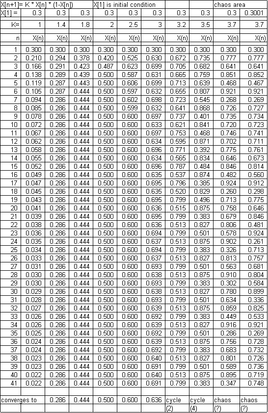
Below is a copy of a spreadsheet that illustrates chaotic behavior. The math is described on page 35 of REASON AND REALITY by John Polkinghorne (1991) and describes how species population sizes vary in successive years. Next year’s population (X[n+1]} depends on:

(1) how many of the species there are to breed this year (X[n])

(2) on the attenuating effect of limited resources this year (1-X[n]).

X is a scaled population size and K is the coupling effect determining how strong these two factors are in determining actual population size.  Note the results through a 41 year cycle of various values of K. X[1] may be set to any value more than 0 and less than 1. If K=2 the value quickly settles down to 0.5 after a few years. For K=3.2 there is a two cycle oscillation. By K=3.58 no stable pattern is ever established. Chaos.

So what? A simple equation can produce unpredictable behavior. Try, for example, with K = 3.7, both X[1} = 0.3 and X[1] = 0.3001. At first the predicted values are similar – then wide divergence. This is true for even values of K which differ from one another by only a few millionths of a percent. We can never know initial conditions accurately enough to predict far into the future. The application is evident when applied to weather forecasting, of course.